Why Error Corection is never as clear as its seems
Throughout my short technical career, I have frequently felt the need to use some form of Error correction either to protect data transmitted over a noisy medium or as an additional safeguard for long-term stored data. The used Error Correction was always some sort of CRC. Unfortunately, I was never fully confident about which algorithm to choose, which polynomial was most appropriate, or how large the protected data could be relative to the CRC size for the checksum to remain meaningful.Perhaps you have faced the same questions and wondered how the different parameters of the mysterious CRC algorithm influence its effectiveness. In this short article, I would like to invite you to follow my line of thinking on this topic. Be warned, however: there are likely some flaws or misconceptions hidden along the way, waiting to be discovered.
The story of Error Correction
First of all, I would like to start this journey by explaining what a CRC actually is and why it exists. If you think of a data transfer between two communication devices, it is essentially a sequence of binary data. On one side, there is a communication device sending data over an unknown medium, such as cables or even electromagnetic waves through the air, and on the other side, there is a receiver receiving this stream of data.In this communication model, the sender continuously transmits data to the receiver, and the receiver interprets the received data and acts according to it. As an example, consider a digital temperature sensor that continuously sends its measurement data, and a receiver that interprets this data and possibly reacts to it. For instance, the receiver may shut down the system if the temperature becomes too high in order to prevent damage.
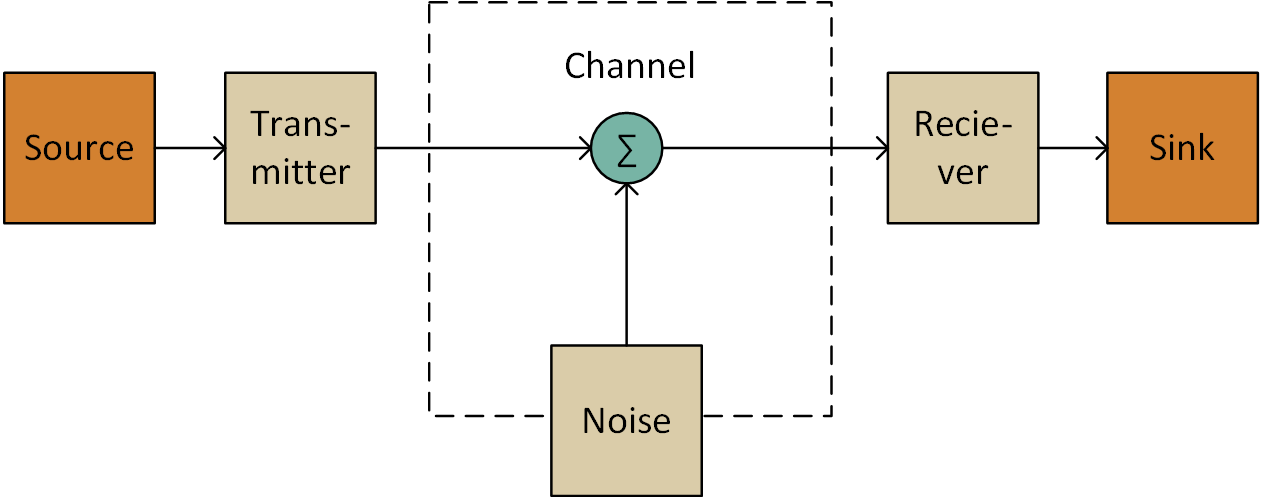
If the communication medium were perfect and completely free of noise, this communication would work without any issues. The sender would continuously transmit the measured temperature, and the receiver would receive and interpret it correctly. However, once we consider real-world systems, we must introduce noise into the communication channel (this is visualized in the famous figure by Shannon shown on the right).
To better understand noise and its effect on the data stream, it is helpful to simplify the communication model. In this simplified view, the transmission of a 1 bit is represented as a signal on the medium, while a 0 bit is represented by the absence of a signal. This communication method is easy to implement and is commonly used in wired communication systems.
By focusing on the 0 bit, the effect of noise becomes easier to visualize. When the sender stops transmitting and a 0 bit is intended to be sent, the data stream leaves the sender and enters the medium. In the medium, it is affected by noise before being received by the receiver. If the noise level at that moment is high enough, the receiver may falsely interpret the noise as a 1 bit and thus misinterpret the received data. Hurray — we have our first error.
So how do we handle errors on the receiver side, and how do we detect them? Moreover, how do we detect errors when the receiver cannot send any packets back to the sender? The simplest approach to detect errors is to repeat the message. By comparing the received messages, it is possible to determine whether an error occurred or if the message is correct. Naturally, this approach doubles the amount of transmitted data, since the message has to be sent twice.
Now, consider what happens if the message gets corrupted at the exact same position in both transmissions. Yes, that would be a bummer — although it is very unlikely to happen. To mitigate such a scenario, additional redundant data must be added. This simply shifts the likelihood of an undetected error to a much less probable case, and this process can, in principle, be repeated indefinitely.
However, this is not our main interest. It mainly tells us that the amount of redundant data must be chosen according to the expected failure rate. A higher noise level, and therefore a higher failure rate, requires greater redundancy in order to achieve the same probability of falsely verifying an incorrect message.
However, let us focus again on the amount of data required for error detection. By sending the message twice, it was necessary to add redundant data equal to the size of the original message. This is quite a lot of overhead just to detect whether a message is correct or not. Therefore, it would be beneficial to develop a better concept for error detection.
Mathematically, we need a function that uses all input data of our message and converts it into a smaller chunk of data that is appended at the end. The simplest example of such a function is a parity check. This function outputs 1 if the number of ones in the message is odd and 0 if the number is even.
For example, consider the message 010101011010. The number of ones in this message is six, which is an even number, so the parity bit is 0. This parity bit is then appended to the message, allowing the receiver to perform exactly the same simple test to verify its content.
Technically, such a parity function has the benefit that it can be implemented very easily as a
chain of XOR operations over all individual data bits in the message. This makes it fast and simple. Sounds nice,
doesn't it?
Of course, a one-bit overhead solution for everything sounds too good to be true — and sadly, it is. The drawback of this approach is that only single-bit errors are guaranteed to be detected; certain multi-bit errors may remain undetected. For instance, if two zeros are flipped to ones within the message, the parity does not change, and the error goes unnoticed.
Let us try this with our known message:
To get an idea of the main reason behind this problem, we have to take a closer look at the mathematics involved. For this purpose, we consider a mathematical set. A mathematical set is simply a collection of elements — in our case, all possible messages exchanged between the sender and the receiver.
These messages may contain actual temperature values, synchronization information, configuration data, and so on. All these unique bit patterns can be grouped into a single set. For this set, we can define a function (for example, the parity function). When we apply this function to any element of the set, we obtain an output — mathematically referred to as the image.
Of course, a one-bit overhead solution for everything sounds too good to be true — and sadly, it is. The drawback of this approach is that only single-bit errors are guaranteed to be detected; certain multi-bit errors may remain undetected. For instance, if two zeros are flipped to ones within the message, the parity does not change, and the error goes unnoticed.
Let us try this with our known message:
- No flip: 010101011010 → parity 0 → no parity error
- One flip: 110101011010 → parity 0 → parity error detected
- Two flips: 110111011010 → parity 0 → no parity error
To get an idea of the main reason behind this problem, we have to take a closer look at the mathematics involved. For this purpose, we consider a mathematical set. A mathematical set is simply a collection of elements — in our case, all possible messages exchanged between the sender and the receiver.
These messages may contain actual temperature values, synchronization information, configuration data, and so on. All these unique bit patterns can be grouped into a single set. For this set, we can define a function (for example, the parity function). When we apply this function to any element of the set, we obtain an output — mathematically referred to as the image.

In the case of parity, this image consists of only two possible values: zero and one. This means that all possible messages are mapped to just two different results. The ratio between the number of elements in the input set and the number of elements in the output set essentially defines the compression ratio. However, as this ratio becomes larger and larger, the error immunity becomes worse and worse.
So, to achieve good error detection, we need a function that produces the right number of error-detection codes in its image to remain efficient. As an additional technical requirement, this function must also be implementable in hardware and should be fast and cheap. In other words, we are looking for the standard “impossible” solution.
The resolution to this problem is essentially the CRC algorithm. It can be implemented very easily in hardware and is fast and cheap to realize. The algorithm is based on polynomial division: the input message is divided by a given polynomial, and the remainder is used as a checksum. This is conceptually similar to parity checking if the division is performed with the polynomial x+1.
This marks the starting point of my journey: how do we choose the polynomial, and does it really make that much of a difference?
If we recall the idea of sets and the function between them, we may get a clue as to which polynomial should be chosen. The key observation is that, for a given set of input messages, it is not strictly necessary that all possible elements of the output set are reachable by the function. In other words, some output values may be impossible to produce. A similar principle applies to the input set as well.
Therefore, it is beneficial to maximize the distance between different members of a set. By distance, I mean the so-called Hamming distance, which is the number of bit flips required to transform one element into another. For example, consider the following two messages:
- 010101011010
- 110111011010
Hurray — have we found our solution? But how do we select such a polynomial for our function? This is actually where the struggle begins. Since I am currently not fully aware of a systematic solution to this problem (work in progress), I created a simple application to help explore and solve it for me.
The application is a simple, multiprocessed Python program that calculates the number of falsely accepted messages for a given input message containing n bit errors. Additionally, it computes the Hamming distance of the error patterns in the falsely validated messages. For instance the Polynom 5B created following results:
| Error 1 | Error 2 | Error 3 | Error 4 | Error 5 | Error 6 | Error 7 | |
|---|---|---|---|---|---|---|---|
| Done | 64 | 2016 | 41664 | 635376 | 7624512 | 74974368 | 621216192 |
| Error | 0 | 0 | 333 | 5043 | 59537 | 585949 | 4853031 |
| MAX D | 0 | 0 | 63 | 63 | 63 | 63 | 63 |
| Min D | 1 | 1 | 1 | 1 | 1 | ||
| MED D | 22.016016016016014 | 19.457348985910865 | 21.33952776500924 | 21.658525431639763 | 21.662783319581518 |
| Error 1 | Error 2 | Error 3 | Error 4 | Error 5 | Error 6 | Error 7 | |
|---|---|---|---|---|---|---|---|
| Done | 64 | 2016 | 41664 | 635376 | 7624512 | 74974368 | 621216192 |
| Error | 0 | 0 | 0 | 5036 | 0 | 586130 | 0 |
| MAX D | 0 | 0 | 0 | 63 | 0 | 63 | 0 |
| Min D | 1 | 1 | |||||
| MED D | 19.448267366027864 | 21.6576827519158 |
The results show that, depending on the chosen polynomial and the distance between the error bits, the outcomes can vary massively.
The application which calculates this tables is visible on GitHub.